
Methodology document
Satellite image data processing at Statistics Canada for the Crop Condition Assessment Program (CCAP)
For: Statistics Canada Integrated Metadata base
Written by: Frédéric Bédard
Reviewed by: Richard Dobbins, Gordon Reichert
Remote Sensing and Geospatial Analysis (RSGA)
Agriculture Division
Statistics Canada
April 2010
Background
Data processing steps
Time required for Web application update
References
1. Background
Interactive and available free of charge via the Internet (http://www26.statcan.ca/ccap-peec), the Crop Condition Assessment Program (CCAP) uses low-resolution, satellite image data during the crop growing season to monitor changing vegetation conditions throughout the entire agricultural region of Canada as well as the northern portion of the United States.
CCAP’s main data source is raw satellite imagery. The application can be launched using two different satellite image data sources. The original application uses 1-kilometer resolution data obtained from the Advanced Very High Resolution Radiometer (AVHRR) of the National Oceanic and Atmospheric Administration (NOAA) series of Earth observation (EO) satellites. A new application launched in 2010 uses 250-meter resolution satellite image data obtained from the Moderate Resolution Imaging Spectroradiometer (MODIS), onboard the TERRA experimental satellite.
This document describes the data processing steps performed at Statistics Canada for the release of data via the CCAP. Prior to these steps, weekly 7-day composite images are built from daily raw satellite image data processed by our partners. NOAA-AVHRR weekly 7-day image composites are built using software developed by the Canada Center for Remote Sensing (CCRS), Natural Resources Canada (NRCan). This general data processing methodology is described in Latifovic et al. (2005). The TERRA-MODIS image composites are built by a team of the Agri-Environmental Data group from Agriculture and Agri-Food Canada (AAFC) (Davidson et al., 2009).
2. Data processing steps
2.1. Processing input weekly composite satellite image data
2.1.1. Input data – AVHRR
These data are received at Statistics Canada via ftp pull in the form of a compressed package containing the following files:
Name of file: CISYYwkWW.zip, where YY is the year (last two digits) and WW is the Julian week number
Individual files:
- B01_retoa.img: channel 1 data, reflectance at top of atmosphere
- B02_retoa.img: channel 2 data, reflectance at top of atmosphere
- Ndvi_retoa.img: Normalized Difference Vegetation Index (NDVI) data, from reflectance at top of atmosphere data
- Comp.log: metadata on output from compositing process
The imagery is received in plain raster format in unsigned integers. During the creation of the composite, NDVI values have been rescaled from the range [-1; 1] to [0; 20 000], using the following formula:
NDVI_rescaled = (NDVI_original * 10 000) + 10 000
Rescaling allows the image data to be saved as integer values instead of real values, with the goal of saving disk space and speed up further processing.
For subsequent steps, only the NDVI channel is used. The B01 and B02 files are individual channel data used to create the NDVI ratio (channel 1 and 2).
The composite data received at Statistics Canada use the following projection parameters:
- Projection type: Lambert conformal conic
- Central meridian: 95° West
- Reference latitude: 0°
- 1st standard parallel: 49° North
- 2nd standard parallel: 77° West
- False Northing: 0
- False Easting: 0
- Earth model: 1980 Geodetic reference system (GRS80)
The output images and maps also use these same projection parameters, so that no geographic re-projection is performed on the source images. The coverage of the source images uses the following (Lambert conformal conic projection coordinates):
- Northwest corner: -2,600,000 East, 10,500,000 North
- Southeast corner: 3,100,000 East, 5,700,000 North
- Spatial resolution (X and Y): 1,000 meters
- Number of pixels: 5,700 columns, 4,800 lines
The entire image is processed for subsequent steps.
Raw AVHRR-NDVI for Julian week 30, 2009
2.1.2. Input data – MODIS
This data is received at Statistics Canada via ftp pull in the form of a compressed package containing the following files:
Name of file: ncomYYYYDDDtoddd.zip, where YYYY is the year, DDD and ddd are the first and last Julian day of the composite period.
Files:
- ncomYYYDDDtoddd.tif: image data in GeoTIFF format
- ncomYYYDDDtoddd.rrd: overview images of the TIF image (to increase speed when image is viewed at small scale)
- ncomYYYDDDtoddd.aux: auxiliary file of the GeoTIFF file
- ncomYYYDDDtoddd.tif.xml: TIF image metadata
NDVI values are stored in real format with values ranging from -1 to 1.
The composite data received at Statistics Canada use the following projection parameters
- Projection type: Sinusoidal
- Earth model: sphere, radius of 6,371,007.181 meters
The coverage and resolution of the source composite image use the following (coordinates in sinusoidal projection):
- Northwest corner: -10,007,554.700 East, 6,671,703.120 North
- Southeast corner: -3,335,851.590 East, 4,447,802.083 North
- Spatial resolution (X and Y): 231.656 meters
- Number of pixels: 28,800 columns, 9,600 lines
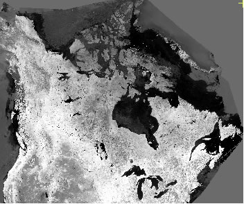
Raw MODIS-NDVI, Julian week 34, 2009
2.2 Reprojection and clipping – MODIS imagery
Geographic image re-projection and clipping is required only for the MODIS image composites. The sinusoidal projection of the input data is used for storing the MODIS imagery at the Land Processes Distributed Active Archive Center (LP-DAAC) in the United States. This projection is not appropriate for displaying imagery over Canada. The composite data therefore needs to be re-projected.
To be consistent with the NOAA AVHRR application, the MODIS imagery is re-projected to the same geographic projection that is used for the AVHRR data (projection parameters described in section 2.1.1.). This allows displaying of maps and images that are comparable when superimposed or viewed side by side.
To reduce the size of files, output images are clipped restricting coverage to only the Canadian land portion where agriculture data is available (south of the 60th parallel).
After the re-projection process, the images are reduced to the following coverage (in Lambert conformal conic projection coordinates)
- Northwest corner: -2,350,000 East, 8,200,000 North
- Southeast corner: 3,020,040 East, 5,755,100 North
- Spatial resolution (X and Y): 230 meters (originally 250 meters in average during acquisition, received at 231.656 m, resampled at 230 meters)
- Number of pixels: 23,348 columns, 10,630 lines
The imagery is rescaled to 16-bit unsigned integer values in order to save disk space and speed up the remaining processing steps. To store the real value in integers, the following formula is applied to all pixel values:
NDVI_rescaled = (NDVI_real * 10,000) + 10,000
Using this process, the image size of each individual composite is reduced from 947 to 473 megabytes, while still maintaining quality and accuracy of the data. Prior to re-projection and clipping, the size of the original imagery is 1.1 gigabyte per composite.
For viewing graphs and tables in the web application, NDVI values are still displayed as real values from -1 to 1.
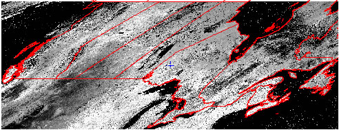
MODIS NDVI re-projected and clipped, Julian week 34, 2009
2.3. Cloud detection and removal
For both the AVHRR and MODIS image composites Statistics Canada completes a cloud and other atmospheric residual contaminants detection. For this work, an in-house application, developed by the Remote Sensing and Geospatial Applications (RSGA) Section, using Visual Studio .Net 2005 and the EASI programming language associated with PCI Geomatica software, version 10.1 is used.
The vegetation index values usually follow a progressive curve, showing an increase at the beginning of the growing season, then levels off in the middle of the summer, and finally decreasing at the end of the growing season. Each pixel (picture element) of the AVHRR image data covers one square kilometre. Since the average field size in Canada is often smaller than one kilometre, each pixel describes the average vegetation vigour of all fields within the pixel. In contrast, MODIS data has a pixel resolution of 250 square meters, therefore a single MODIS pixel will sometimes contain a single crop type or field. The change of NDVI values will usually be progressive, because even if a field is cut during one week, the remaining fields in the pixel will also influence the value of the resulting NDVI and will result in an average that will not fluctuate suddenly. Following the same idea, a field turns green in a matter of weeks, so again progressive change should be observed from week to week at the beginning of the season. And in the worst case, if all fields inside one pixel are cut, the NDVI value will decrease rapidly but the values will remain low for at least a few weeks.
Based on these facts, a pixel will be considered contaminated if a sudden drop is immediately followed by a sudden increase in the following week.
In order not to have to wait for the following week to make a correction, a first detection will be made by comparing values of the current week with the previous week. The pixel will be corrected by repeating the value of the previous week if a NDVI value declines more than 0.05 from week 15 to 28 (where values should normally increase or remain stable), or more than 0.20 from week 29 to the end of the season. The threshold is higher after the normal peak of the NDVI values because at that time it is normal to observe larger drops in values because annual crops are ripening and fields are being harvested.
Upon reception of the following week’s imagery, cloud detection and correction is performed again on the original values. The pixel will be identified as contaminated if a NDVI value drop of more than 0.01 is followed by an increase of at least 0.01.
For now, no correction is applied if atmospheric contamination is present for two or more consecutive weeks, because this requires a minimum of 4 weeks of data to perform, which is difficult to operate in near-real time conditions.
Statistical imputation is employed when a pixel was identified as contaminated. The imputation method used is the following:
- when the following week is not available, pixel values are temporarily replaced by the value of the previous week
- when the following week is available, the current value will be replaced by the average NDVI value of the previous and the following week
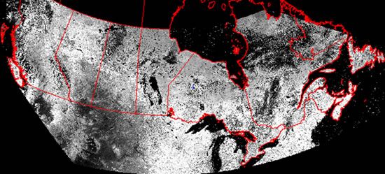
Raw MODIS-NDVI, entire image, Julian week 34, 2009

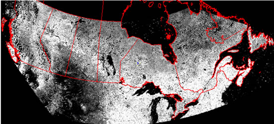
Cloud-corrected NDVI, entire image, Julian week 34, 2009
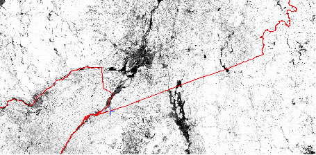
Raw MODIS-NDVI, Ottawa-Montreal area, Julian week 34, 2009
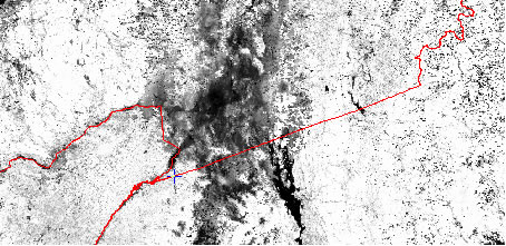
Cloud-corrected MODIS-NDVI, Ottawa-Montreal area, Julian week 34, 2009
2.4. Computing statistics by region
For thematic mapping, preliminary statistics are computed and stored in a relational database for each new week received, and for each geography layer available.
Geographic layers displayed via the CCAP include:
- Census Agriculture Regions (CAR);
- Census Divisions (CD);
- Census Consolidated Subdivisions (CCS) – municipalities;
- Townships (for Prairies only);
- Counties, (for the United States portion only).
Only pixels identified as mainly covered by agriculture are used in the calculations. This allows the application to display variations in NDVI for crop and pasture conditions only, aside from other land cover types that might influence the NDVI in a different way (for example, forests, water bodies or urban areas).
A land cover database in image format for the entire agriculture area of Canada was built by Agriculture and Agri-Food Canada, using 2000 as the reference year. This database was built using medium-resolution (Landsat) satellite data. This product, as well as metadata, is available at (http://www.geobase.ca/geobase/en/data/landcover/index.html.)
Three different filters are available in the CCAP application. An agriculture filter was built by selecting 1 square kilometre pixels (AVHRR application) or 250-meter pixels (MODIS application) covered by at least 50% of the sum of classes 110 (grassland), 120 (cultivated agriculture land), 121 (annual cropland) and 122 (perennial cropland and pasture) as defined within the AAFC Landsat classification referenced above.
The crops filter was built using the same method but using only the sum of classes 121 and 122. The grassland or pasture filter uses class 110. Pasture in this case refers to natural pasture or grassland. Since this land cover type is very rarely represented in the eastern Canada (from Ontario to Newfoundland-and-Labrador) and eastern United States, only the “total agriculture” layer has been built for these areas. In Canada, the cropland and pasture masks are only available for the provinces of British Columbia, Alberta, Saskatchewan and Manitoba.
For the United States portion, land cover data from the National Land Cover Database, available at http://www.mrlc.gov, is used. This database was built using medium-resolution satellite data. The reference year for this database is 2001. Masks are built using the same method as the Canadian portion. The cropland mask is built using pixels where class 81 (Pasture and hay) or 82 (cultivated crops) are dominant (> 50% of pixel). The grassland or pasture mask is built where class 71 (grassland and herbaceous) covers more than 50% of the pixel. The agriculture mask is built where the combination of these three classes is dominant (>50%) for an pixel. In areas east of the Great Plains, only the total agriculture mask is used.
For the Canadian Prairies and the US Great Plains, three average NDVI values per week are computed for each geography layer: total agriculture, cropland only, pasture (grassland) only. For the remaining area, averages are calculated only using the agriculture filter.
Once average NDVI values are computed, they are exported to a relational database. The web application creates a live link with this database, and values are queried to create thematic maps, graphics and tables “on-the-fly”.
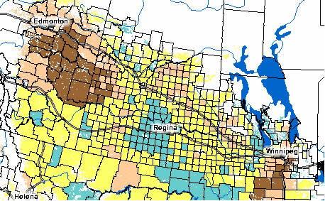
Example of thematic map: Average AVHRR NDVI by municipality (CCS) for Julian week 27, 2009 over the Canadian Prairies
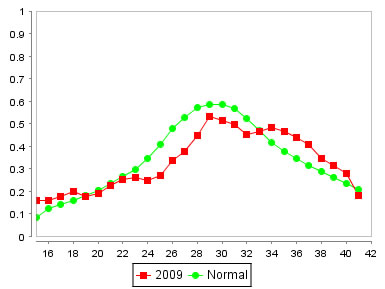
Example of graphic: Current year AVHRR-NDVI compared to normal Flagstaff, Alberta (CCS 4807031)
Julian weeks |
2009 |
2009 Dates |
Normal |
2009 - Normal |
|---|---|---|---|---|
15 |
0.1592 |
April 6 to 12, 2009 |
0.1127 |
0.0465 |
16 |
0.1602 |
April 13 to 19, 2009 |
0.1394 |
0.0208 |
17 |
0.1764 |
April 20 to 26, 2009 |
0.1537 |
0.0226 |
18 |
0.2005 |
April 27 to May 3, 2009 |
0.1736 |
0.0269 |
19 |
0.175 |
May 4 to 10, 2009 |
0.1953 |
-0.0203 |
20 |
0.1894 |
May 11 to 17, 2009 |
0.2215 |
-0.0321 |
21 |
0.2232 |
May 18 to 24, 2009 |
0.253 |
-0.0298 |
22 |
0.2504 |
May 25 to 31, 2009 |
0.2847 |
-0.0342 |
23 |
0.2605 |
June 1 to 7, 2009 |
0.3227 |
-0.0622 |
24 |
0.2449 |
June 8 to 14, 2009 |
0.3783 |
-0.1334 |
25 |
0.2695 |
June 15 to 21, 2009 |
0.4443 |
-0.1747 |
26 |
0.3359 |
June 22 to 28, 2009 |
0.509 |
-0.1731 |
27 |
0.3775 |
June 29 to July 5, 2009 |
0.5545 |
-0.177 |
28 |
0.4475 |
July 6 to 12, 2009 |
0.5727 |
-0.1252 |
29 |
0.5312 |
July 13 to 19, 2009 |
0.5837 |
-0.0525 |
30 |
0.5135 |
July 20 to 26, 2009 |
0.5752 |
-0.0617 |
31 |
0.4957 |
July 27 to August 2, 2009 |
0.5385 |
-0.0428 |
32 |
0.454 |
August 3 to 9, 2009 |
0.4915 |
-0.0375 |
33 |
0.4638 |
August 10 to 16, 2009 |
0.4378 |
0.026 |
34 |
0.4846 |
August 17 to 23, 2009 |
0.3968 |
0.0877 |
35 |
0.465 |
August 24 to 30, 2009 |
0.3544 |
0.1105 |
36 |
0.4376 |
August 31 to September 6, 2009 |
0.3241 |
0.1135 |
37 |
0.4081 |
September 7 to 13, 2009 |
0.2973 |
0.1109 |
38 |
0.344 |
September 14 to 20, 2009 |
0.2719 |
0.0721 |
39 |
0.3127 |
September 21 to 27, 2009 |
0.244 |
0.0687 |
40 |
0.2777 |
September 28 to October 4, 2009 |
0.218 |
0.0597 |
41 |
0.1804 |
October 5 to 11, 2009 |
0.1906 |
-0.0102 |
When the following week is available, new NDVI averages are calculated for the reference week, because more accurate cloud detection is applied to the imagery to increase the accuracy of the NDVI values as explained in section 2.3.
2.5. Creating image products
The CCAP does not display raw NDVI composites on the application. Raw NDVI values have very limited use unless they are compared with other values.
When displayed on the web application, the images and maps are classified into 5 distinct classes:
Classes for images and maps
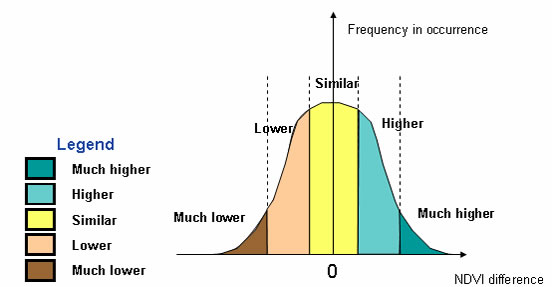
For each individual product described in the following subsections, thresholds (range cutoffs) have been established. These cutoffs are based on how a certain value differs statistically from another comparison value. This analysis is based on a normal distribution of difference values. The following table specifies the thresholds for each product.
| Compared to normal | Compared to previous year | |||
|---|---|---|---|---|
| Class | minimum | maximum | minimum | maximum |
| Much higher | --- | -0.0876 | --- | -0.3283 |
| Higher | -0.0875 | -0.0292 | -0.3282 | -0.1095 |
| Similar | -0.0291 | 0.0291 | -0.1094 | 0.1094 |
| Lower | 0.0292 | 0.0875 | 0.1095 | 0.3283 |
| Much lower | 0.0876 | --- | 0.3284 | --- |
| Compared to previous week | Compared to highest value of normal | |||
|---|---|---|---|---|
| Class | minimum | maximum | minimum | maximum |
| Much higher | --- | -0.2783 | --- | -0.1323 |
| Higher | -0.2782 | -0.0928 | -0.1322 | -0.0441 |
| Similar | -0.0927 | 0.0927 | -0.0440 | 0.0440 |
| Lower | 0.0928 | 0.2782 | 0.0441 | 0.1322 |
| Much lower | 0.2783 | --- | -0.1323 | --- |
The CCAP provides comparisons with the following four reference images.
2.5.1. Comparing current NDVI values with the historical normal values
The AVHRR database includes NDVI 7-day composite data from 1987 to present. The MODIS database includes imagery from 2000 to present. A normal image file is created pixel by pixel for each of the Julian weeks available in the application (15 to 41 for the AVHRR, 15 to 37 for the MODIS).
At the end of a growing season, normal images are updated by adding the most recent year of data to calculate the new normal values that will be used for the following year. New normal averages by geographic regions are also computed at that time to update the database.
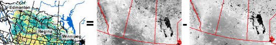
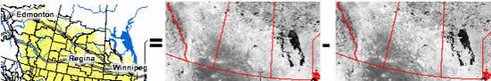
When a user requests a comparison of the current NDVI values with the normal, the operation is achieved by doing a simple subtraction calculation and the results displayed as depicted in Image product 1:
Image product 1 (Compared to normal) = NDVI_weekWW_currentyear – NDVI_weekWW_normal (where WW is the Julian week of the image)
Example with week 34, 2009 (AVHRR NDVI)
2.5.2. Comparing with previous year
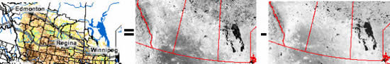
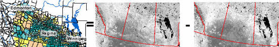
The second image product compares NDVI values of a specified week with the same week of the previous year.
Image product 2 (compare to previous year) = NDVI_weekWW_currentyear – NDVI_weekWW_previousyear (where WW is the Julian week of the image)
Example with week 34, 2009 (AVHRR NDVI)
2.5.3. Comparing with previous week
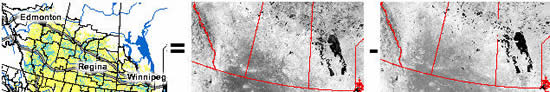
The third image product compares NDVI values of a specified week with values of the previous week (same year).
Image product 3 (compare to previous week) = NDVI_weekWW – NDVI_week(WW-1) (where WW is the Julian week of the image.)
Example with week 34, 2009 (AVHRR NDVI)
2.5.4. Comparing with highest value of normal
The fourth image product allows users to compare NDVI values of a specified week with the highest NDVI values for a given region. These highest NDVI values are normally reached in mid-summer, the peak of the growing season. Since the NDVI peak does not always occur during the same week each year, this product allows users to compare values of any week against the historic normal peak.
When the normal data and images are updated, the maximum values of the normal are updated also on a pixel by pixel basis. Average maximum NDVI by region is recomputed and stored in the database when normal data are reprocessed.
Image product 4 (compare with highest value of normal) = NDVI_weekWW – NDVI_highestvalueofnormal (where WW is the Julian week of the image.)
Example with week 34, 2009 (AVHRR NDVI)
2.5.5. Comparing with any other week
Regarding the production of CCAP thematic maps, NDVI values generated for any week and in any year, can be compared against any other week of any other year. NDVI data from the two periods which are specified by the user are subtracted and classified.
Thematic map, compare any week of any year
Week 31, 2003, compared with week 31, 1988 (AVHRR NDVI)
2.6. Update web application
When all data processing is complete, the web application is temporarily shut down but usually for only a few minutes. Operations that need to be accomplished during the maintenance are:
- Update of the database;
- Addition of new imagery;
- Update of application parameter file. This file informs the application what data to display when the application is launched. By default, the application opens always by showing the most recent NDVI image compared with the normal
3. Time required for Web application update
The following table displays the complete data processing steps with time required to complete each step.
Step |
AVHRR NDVI |
MODIS NDVI |
|---|---|---|
Creation of composite (done outside of Statistics Canada) |
0.5 day after end of composite period (Monday afternoon) |
4 - 5 days after end of composite period (late Thursday to Friday) |
Downloading image through FTP |
1 hour |
2 hours |
Image reprojection, resampling and clipping |
Not applicable |
1h15m |
Cloud detection and removal |
5 minutes |
20 min |
Computing statistics by region and database update |
10 minutes |
25 min |
Creation of Image products |
5 minutes |
2 hours |
Quality control |
30 minutes |
1 hour |
File transfer to server and update |
15 minutes |
1 hour |
TOTAL TIME |
0.7 day after end of composite period |
4 - 7 days after end of composite period |
Update time (earliest) |
Monday 2:00 pm |
Friday 4:00 pm, but more likely afternoon of the following Monday |
4. References
Davidson A., Howard A., Sun, K., Pregitzer M., Rollin, P., Aly Z. (2009) A National Crop Monitoring System prototype (NCMS-P) using MODIS data: Near-Real-Time Agricultural Assessment from Space. Agriculture and Agri-food Canada, National Land and Water Information Service, 41 p.
Latifovic, R., Trishchenko, A. P., Chen J., Park W.B., Khlopenkov, K. V., Fernandes, R., Pouliot, D., Ungureanu, C., Luo, Y., Wang, S., Davidson, A., Cihlar, J. (2005) Generating historical AVHRR 1 km baseline satellite data records over Canada suitable for climate change studies. Canadian Journal of Remote Sensing, vol. 31, no 5, pp 324-346.
- Date modified: